Hemodynamic Deconvolution Demystified: Sparsity-Driven Regularization at Work
Abstract
Deconvolution of the hemodynamic response is an important step to access short timescales of brain activity recorded by functional magnetic resonance imaging (fMRI). Albeit conventional deconvolution algorithms have been around for a long time (e.g., Wiener deconvolution), recent state-of-the-art methods based on sparsity-pursuing regularization are attracting increasing interest to investigate brain dynamics and connectivity with fMRI. This technical note revisits the main concepts underlying two main methods, Paradigm Free Mapping and Total Activation, in the most accessible way. Despite their apparent differences in the formulation, these methods are theoretically equivalent as they represent the synthesis and analysis sides of the same problem, respectively. We demonstrate this equivalence in practice with their best-available implementations using both simulations, with different signal-to-noise ratios, and experimental fMRI data acquired during a motor task and resting-state. We evaluate the parameter settings that lead to equivalent results, and showcase the potential of these algorithms compared to other common approaches. This note is useful for practitioners interested in gaining a better understanding of state-of-the-art hemodynamic deconvolution, and aims to answer questions that practitioners often have regarding the differences between the two methods.
Keywords:
fMRI deconvolution, paradigm free mapping, total activation, temporal regularization
1. Introduction
Functional magnetic resonance imaging (fMRI) data analysis is often directed to identify and disentangle the neural processes that occur in different brain regions during task or at rest. As the blood oxygenation level-dependent (BOLD) signal of fMRI is only a proxy for neuronal activity mediated through neurovascular coupling, an intermediate step that estimates the activity-inducing signal, at the timescale of fMRI, from the BOLD timeseries can be useful. Conventional analysis of task fMRI data relies on the general linear models (GLM) to establish statistical parametric maps of brain activity by regression of the empirical timecourses against hypothetical ones built from the knowledge of the experimental paradigm. However, timing information of the paradigm can be unknown, inaccurate, or insufficient in some scenarios such as naturalistic stimuli, resting-state, or clinically-relevant assessments.
Deconvolution and methods alike are aiming to estimate neuronal activity by undoing the blurring effect of the hemodynamic response, characterized as a hemodynamic response function (HRF)
Deconvolution of the resting-state fMRI signal has illustrated the significance of transient, sparse spontaneous events (Petridou et al., 2012; Allan et al., 2015) that refine the hierarchical clusterization of functional networks (Karahanoglu et al., 2013) and reveal their temporal overlap based on their signal innovations not only in the human brain (Karahanoğlu and Ville, 2015), but also in the spinal cord (Kinany et al., 2020). Similar to task-related studies, deconvolution allows to investigate modulatory interactions within and between resting-state functional networks (Di and Biswal, 2013, 2015). In addition, decoding of the deconvolved spontaneous events allows to decipher the flow of spontaneous thoughts and actions across different cognitive and sensory domains while at rest (Karahanoğlu and Ville, 2015; Gonzalez-Castillo et al., 2019; Tan et al., 2017). Beyond findings on healthy subjects, deconvolution techniques have also proven its utility in clinical conditions to characterize functional alterations of patients with a progressive stage of multiple sclerosis at rest (Bommarito et al., 2020), to find functional signatures of prodromal psychotic symptoms and anxiety at rest on patients suffering from schizophrenia (Zöller et al., 2019), to detect the foci of interictal events in epilepsy patients without an EEG recording (Lopes et al., 2012; Karahanoglu et al., 2013), or to study functional dissociations observed during non-rapid eye movement sleep that are associated with reduced consolidation of information and impaired consciousness (Tarun et al., 2020).
The algorithms for hemodynamic deconvolution can be classified based on the assumed hemodynamic model and the optimization problem used to estimate the neuronal-related signal. Most approaches assume a linear time-invariant model for the hemodynamic response that is inverted by means of variational (regularized) least squares estimators (Glover, 1999; Gitelman et al., 2003; Gaudes et al., 2010, 2012, 2013; Caballero-Gaudes et al., 2019; Hernandez-Garcia and Ulfarsson, 2011; Karahanoğlu et al., 2013; Cherkaoui et al., 2019; Hütel et al., 2021; Costantini et al., 2022), logistic functions (Bush and Cisler, 2013; Bush et al., 2015; Loula et al., 2018), probabilistic mixture models (Pidnebesna et al., 2019), convolutional autoencoders (Hütel et al., 2018) or nonparametric homomorphic filtering (Sreenivasan et al., 2015). Alternatively, several methods have also been proposed to invert non-linear models of the neuronal and hemodynamic coupling (Riera et al., 2004; Penny et al., 2005; Friston et al., 2008; Havlicek et al., 2011; Aslan et al., 2016; Madi and Karameh, 2017; Ruiz-Euler et al., 2018).
Among the variety of approaches, those based on regularized least squares estimators have been employed more often due to their appropriate performance at small spatial scales (e.g., voxelwise). Relevant for this work, two different formulations can be established for the regularized leastsquares deconvolution problem, either based on a synthesis- or analysis-based model (Elad et al., 2007; Ortelli and van de Geer, 2019). The rationale of the synthesis-based model is that we know or suspect that the true signal (here, the neuronally-driven BOLD component of the fMRI signal) can be represented as a linear combination of predefined patterns or dictionary atoms (for instance, the hemodynamic response function). In contrast, the analysis-based approach considers that the true signal is analyzed by some relevant operator and the resulting signal is small (i.e., sparse).
As members of the groups that developed Paradigm Free Mapping (synthesis-based solved with regularized least-squares estimators such as ridge-regression Gaudes et al. 2010 or LASSO Gaudes et al. 2013) and Total Activation (analysis-based also solved with a regularized least-squares estimator using generalized total variation Karahanoglu et al. 2011; Karahanoğlu et al. 2013 ) deconvolution methods for fMRI data analysis, we are often contacted by researchers who want to know about the similarities and differences between the two methods and which one is better. It depends—and to clarify this point, this note revisits synthesis- and analysis-based deconvolution methods for fMRI data and comprises four sections. First, we present the theory behind these two deconvolution approaches based on regularized least squares estimators that promote sparsity: Paradigm Free Mapping (PFM) (Gaudes et al., 2013)—available in AFNI as 3dPFM
2. Theory
2.1. Notations and definitions
Matrices of size N rows and M columns are denoted by boldface capital letters, e.g., X ∈ ℝNxM, whereas column vectors of length N are denoted as boldface lowercase letters, e.g., x ∈ ℝN. Scalars are denoted by lowercase letters, e.g., k. Continuous functions are denoted by brackets, e.g., h(t), while discrete functions are denoted by square brackets, e.g., x[k].. The Euclidean norm of a matrix X is denoted as ||X||2, the 𝓵1-norm is denoted by ||X||1 and the Frobenius norm is denoted by ||X|F. The discrete integration (L) and difference (D) operators are defined as:
2.2. Conventional general linear model analysis
Conventional general linear model (GLM) analysis puts forward a number of regressors incorporating the knowledge about the paradigm or behavior. For instance, the timing of epochs for a certain condition can be modeled as an indicator function p(t) (e.g., Dirac functions for event-related designs or box-car functions for block-designs) convolved with the hemodynamic response function (HRF) h(t), and sampled at TR resolution (Friston et al., 1994, 1998; Boynton et al., 1996; Cohen, 1997):
x(t)
=
P
*
h(t)
→
x[k]
=
p
*
h(k
· TR).
The vector x = [x[k]]]k = 1,…,N ∈ ℝN then constitutes the regressor modelling the hypothetical response, and several of them can be stacked as columns of the design matrix X = [x1 … xL] ∈ ℝNxL, leading to the well-known GLM formulation:
y = Xβ + e,(1)
where the empirical timecourse y ∈ ℝN is explained by a linear combination of the regressors in X weighted by the parameters in β ∈ ℝL and corrupted by additive noise e ∈ ℝN. Under independent and identically distributed Gaussian assumptions of the latter, the maximum likelihood estimate of the parameter weights reverts to the ordinary least-squares estimator; i.e., minimizing the residual sum of squares between the fitted model and measurements. The number of regressors L is typically much less than the number of measurements N, and thus the regression problem is over-determined and does not require additional constraints or assumptions (Henson and Friston, 2007).
In the deconvolution approach, no prior knowledge of the hypothetical response is taken into account, and the purpose is to estimate the deconvolved activity-inducing signal s from the measurements y, which can be formulated as the signal model
y = Hs + e,(2)
where H ∈ ℝNxN is a Toeplitz matrix that represents the discrete convolution with the HRF, and s ∈ ℝn is a length-N vector with the unknown activity-inducing signal. Note that the temporal resolution of the activity-inducing signal and the corresponding Toeplitz matrix is generally assumed to be equal to the TR of the acquisition, but it could also be higher if an upsampled estimate is desired. Despite the apparent similarity with the GLM equation, there are two important differences. First, the multiplication with the design matrix of the GLM is an expansion as a weighted linear combination of its columns, while the multiplication with the HRF matrix represents a convolution operator. Second, determining s is an ill-posed problem given the nature of the HRF. As it can be seen intuitively, the convolution matrix H is highly collinear (i.e., its columns are highly correlated) due to large overlap between shifted HRFs (see Figure 2C), thus introducing uncertainty in the estimates of s when noise is present. Consequently, additional assumptions under the form of regularization terms (or priors) in the estimate are needed to reduce their variance. In the least squares sense, the optimization problem to solve is given by
(3)
The first term quantifies data fitness, which can be justified as the log-likelihood term derived from Gaussian noise assumptions, while the second term Ω(s) brings in regularization and can be interpreted as a prior on the activity-inducing signal. For example, the 𝓵2-norm of s (i.e., ) is imposed for ridge regression or Wiener deconvolution, which introduces a tradeoff between the data fit term and “energy” of the estimates that is controlled by the regularization parameter λ. regularized terms are related to the elastic net (i.e., ) [REF].
2.3. Paradigm Free Mapping
In paradigm free mapping (PFM), the formulation of Eq. (3) was considered equivalently as fitting the measurements using the atoms of the HRF dictionary (i.e., columns of H) with corresponding weights (entries of s).. This model corresponds to a synthesis formulation. In Gaudes et al. 2013 a sparsity-pursuing regularization term was introduced on s, which in a strict way reverts to choosing Ω(s) = λ║s║0 as the regularization term and solving the optimization problem (Bruckstein et al., 2009). However, finding the optimal solution to the problem demands an exhaustive search across all possible combinations of the columns of H. Hence, a pragmatic solution is to solve the convex-relaxed optimization problem for the l1-norm, commonly known as Basis Pursuit Denoising (Chen et al., 2001) or equivalently as the least absolute shrinkage and selection operator (LASSO) (Tibshirani, 1996):
(4)
which provides fast convergence to a global solution. Imposing sparsity on the activity-inducing signal implies that it is assumed to be well represented by a reduced subset of few non-zero coefficients at the fMRI timescale, which in turn trigger event-related BOLD responses. Hereinafter, we refer to this assumption as the spike model. However, even if PFM was developed as a spike model, its formulation in Eq.(4) can be extended to estimate the innovation signal, i.e., the derivative of the activity-inducing signal, as shown in section 2.5.
2.4. Total Activation
Alternatively, deconvolution can be formulated as if the signal to be recovered directly fits the measurements and at the same time satisfies some suitable regularization, which leads to
(5)
Under this analysis formulation, total variation (TV), i.e., the 𝓵1 -norm of the derivative Ω(x) = λ║Dx║1, is a powerful regularizer since it favors recovery of piecewise-constant signals (Chambolle, 2004). Going beyond, the approach of generalized TV introduces an additional differential operator DH in the regularizer that can be tailored as the inverse operator of a linear system (Karahanoglu et al., 2011), that is, Ω(x) = λ║DDHx║1. In the context of hemodynamic deconvolution, Total Activation is proposed for which the discrete operator DH is derived from the inverse of the continuous-domain linearized Balloon-Windkessel model (Buxton et al., 1998; Friston et al., 2000). The interested reader is referred to (Khalidov et al., 2011; Karahanoglu et al., 2011; Karahanoğlu et al., 2013) for a detailed description of this derivation.
Therefore, the solution of the Total Activation (TA) problem
(6)
will yield the activity-related signal x for which the activity-inducing signal s = Dhx and the so-called innovation signal u = Ds, i.e., the derivate of the activity-inducing signal, will also be available, as they are required for the regularization. We refer to modeling the activity-inducing signal based on the innovation signal as the block model. Nevertheless, even if TA was originally developed as a block model, its formulation in Eq.(6) can be made equivalent to the spike model as shown in section 2.5.
2.5. Unifying both perspectives
PFM and TA are based on the synthesis- and analysis-based formulation of the deconvolution problem, respectively. They are also tailored for the spike and block model, respectively. In the first case, the recovered deconvolved signal is synthesized to be matched to the measurements, while in the second case, the recovered signal is directly matched to the measurements but needs to satisfy its analysis in terms of deconvolution. This also corresponds to using the forward or backward model of the hemodynamic system, respectively. Hence, it is possible to make both approaches equivalent (Elad et al., 2007)
To start with, TA can be made equivalent to PFM by adapting it for the spike model; i.e., when removing the derivative operator D of the regularizer in Eq. (6), it can be readily verified that replacing in that case x = Hs leads to identical equations and thus both assume a spike model, since H and Dh will cancel out each other (Karahanoglu et al., 2011)
Conversely, the PFM spike model can also accommodate the TA block model by modifying Eq. (4) with the forward model y = HLu + e. Here, the activity-inducing signal s is rewritten in terms of the innovation signal u as s = Lu where the matrix L is the first-order integration operator (Cherkaoui et al., 2019; Uruñuela et al., 2020). This way, PFM can estimate the innovation signal u as follows:
(7)
and becomes equivalent to TA by replacing u = DDhx, and thus adopting the block model. Based on the previous equations (4), (6) and (7), it is clear that both PFM and TA can operate under the spike and block models, providing a convenient signal model according to the different assumptions of the underlying neuronal-related signal. This work evaluates the core of the two techniques; i.e., the regularized least-squares problem with temporal regularization without considering the spatial regularization term originally incorporated in TA. For the remainder of this paper, we will use the PFM and TA formalisms with both spike and block models.
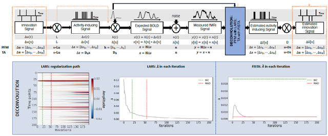
Figure 1: Flowchart detailing the different steps of the fMRI signal and the deconvolution methods described. The orange arrows indicate the flow to estimate the innovation signals, i.e., the derivative of the activity-inducing signal. The blue box depicts the iterative modus operandi of the two algorithms used in this paper to solve the paradigm free mapping (PFM) and total activation (TA) deconvolution problems. The plot on the left shows the regularization path obtained with the least angle regression (LARS) algorithm, where the x-axis illustrates the different iterations of the algorithm, the y-axis represents points in time, and the color describes the amplitude of the estimated signal. The middle plot depicts the decreasing values of λ for each iteration of LARS as the regularization path is computed. The green and r ed dashed lines in both plots illustrate the Bayesian information criterion (BIC) and median absolute deviation (MAD) solutions, respectively. Comparatively, the changes in λ when the fast iterative shrinkage-thresholding algorithm (FISTA) method is made to converge to the MAD estimate of the noise are shown on the right. Likewise, the λ corresponding to the BIC and MAD solutions are shown with dashed lines.
2.6. Algorithms and parameter selection
Despite their apparent resemblance, the practical implementations of the PFM and TA methods proposed different algorithms to solve the corresponding optimization problem and select an adequate regularization parameter λ (Gaudes et al., 2013; Karahanoğlu et al., 2013). The PFM implementation available in AFNI employs the least angle regression (LARS) (Efron et al., 2004), whereas the TA implementation uses the fast iterative shrinkage-thresholding algorithm (FISTA) (Beck and Teboulle, 2009). The blue box in Figure 1 provides a descriptive view of the iterative modus operandi of the two algorithms.
On the one hand, LARS is a homotopy approach that computes all the possible solutions to 154 the optimization problem and their corresponding value of λ; i.e., the regularization path, and 155 the solution according to the Bayesian Information Criterion (BIC) (Schwarz, 1978), was recommended 156 as the most appropriate in the case of PFM approaches since AIC often tends to overfit 157 the signal(Gaudes et al., 2013; Caballero-Gaudes et al., 2019).
On the other hand, FISTA is an extension of the classical gradient algorithm that provides fast convergence for large-scale problems. In the case of FISTA though, the regularization parameter λ must be selected prior to solving the problem, but can be updated in every iteration so that the residuals of the data fit converge to an estimated noise level of the data


:
(8)
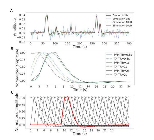
Figure 2: A) Simulated signal with different SNRs (20 dB, 10 dB and 3 dB) and ground truth given in signal percentage change (SPC). B) Canonical HRF models typically used by PFM (solid line) and TA (dashed line) at TR = 0.5 s (blue), TR = 1 s (green) and TR = 2 s (black). Without loss of generality, the waveforms are scaled to unit amplitude for visualization. C) Representation of shifted HRFs at TR = 2 s that build the design matrix for PFM when the HRF model has been matched to that in TA. The red line corresponds to one of the columns of the HRF matrix.
where xn is the nth iteration estimate, λn and λn+1are the nth and n + 1th iteration values for the 159 regularization parameter λ, and N is the number of points in the time-course. The pre-estimated 160 noise level can be obtained as the median absolute deviation (MAD) of the fine-scale wavelet 161 coefficients (Daubechies, order 3) of the fMRI timecourse. The MAD criterion has been adopted 162 in TA (Karahanoğlu et al., 2013). Of note, similar formulations based on the MAD estimate have 163 also been applied in PFM formulations (Gaudes et al., 2012, 2011).
3. Methods
3.1. Simulated data
In order to compare the two methods while controlling for their correct performance, we created a simulation scenario that can be found in the GitHub repository shared in Section 6. For the sake of illustration, we describe here the simulations corresponding to a timecourse with a duration of 400 seconds (TR = 2 s) where the activity-inducing signal includes 5 events, which are convolved with the canonical HRF. Different noise sources (physiological, thermal, and motion-related) were also added and we simulated three different scenarios with varying signal-to-noise ratios (SNR = [20 dB, 10 dB, 3 dB]) that represent high, medium and low contrast-to-noise ratios as shown in Figure 2A. Noise was created following the procedure in (Gaudes et al., 2013) as the sum of uncorrelated Gaussian noise and sinusoidal signals to simulate a realistic noise model with thermal noise, cardiac and respiratory physiological fluctuations, respectively. The physiological signals were generated as
(9)
with up to second-order harmonics per cardiac (fc,i) and respiratory (fr,i) component that were randomly generated following normal distributions with variance 0.04 and mean ifr and ifc, for i = [1, 2]. We set the fundamental frequencies to fr = 0.3 Hz for the respiratory component (Birn et al., 2006)) and fc = 1.1 Hz for the cardiac component (Shmueli et al., 2007)). The phases of each harmonic ϕ were randomly selected from a uniform distribution between 0 and 2π radians. To simulate physiological noise that is proportional to the change in BOLD signal, a variable ratio between the physiological (σp) and the thermal (σ0) noise was modeled as σp/σ0 = a(tSNR)b + c, where a = 5.01 x 10⁻⁶, b = 2.81, and c = 0.397, following the experimental measures available in Table 3 from (Triantafyllou et al., 2005)).
3.2. Experimental data
To compare the performance of the two approaches as well as illustrate their operation, we employ two representative experimental datasets.
Motor task dataset: One healthy subject was scanned in a 3T MR scanner (Siemens) under a Basque Center on Cognition, Brain and Language Review Board-approved protocol. T2*-weighted multi-echo fMRI data was acquired with a simultaneous-multislice multi-echo gradient echo-planar imaging sequence, kindly provided by the Center of Magnetic Resonance Research (University of Minnesota, USA) (Feinberg et al., 2010; Moeller et al., 2010; Setsompop et al., 2011), with the following parameters: 340 time frames, 52 slices, Partial-Fourier = 6/8, voxel size = 2.4 x 2.4 x 3 mm3, TR = 1.5 s, TEs = 10.6/28.69/46.78/64.87/82.96 ms, flip angle = 70o, multiband factor = 4, GRAPPA = 2.
During the fMRI acquisition, the subject performed a motor task consisting of five different movements (left-hand finger tapping, right-hand finger tapping, moving the left toes, moving the right toes and moving the tongue) that were visually cued through a mirror located on the head coil. These conditions were randomly intermixed every 16 seconds, and were only repeated once the entire set of stimuli were presented. Data preprocessing consisted of first, discarding the first 10 volumes of the functional data to achieve a steady state of magnetization. Then, image realignment to the skull-stripped single-band reference image (SBRef) was computed on the first echo, and the estimated rigid-body spatial transformation was applied to all other echoes (Jenkinson et al., 2012; Jenkinson and Smith, 2001). A brain mask obtained from the SBRef volume was applied to all the echoes and the different echo timeseries were optimally combined (OC) voxelwise by weighting each timeseries contribution by its T2* value (Posse et al., 1999). AFNI (Cox, 1996) was employed for a detrending of up to 4th-order Legendre polynomials, within-brain spatial smoothing (3 mm FWHM) and voxelwise signal normalization to percentage change. Finally, distortion field correction was performed on the OC volume with Topup (Andersson et al., 2003), using the pair of spin-echo EPI images with reversed phase encoding acquired before the ME-EPI acquisition (Glasser et al., 2016).
Resting-state datasets: One healthy subject was scanned in a 3T MR scanner (Siemens) under a Basque Center on Cognition, Brain and Language Review Board-approved protocol. Two runs of T2*-weighted fMRI data were acquired during resting-state, each with 10 min duration, with 1) a standard gradient-echo echo-planar imaging sequence (monoband) (TR = 2000 ms, TE = 29 ms, flip-angle = 78o, matrix size = 64 x 64, voxel size = 3 x 3 x 3 mm3, 33 axial slices with interleaved acquisition, slice gap = 0.6 mm) and 2) a simultaneous-multislice gradient-echo echo-planar imaging sequence (multiband factor = 3, TR = 800 ms, TE = 29 ms, flip-angle = 60o, matrix size = 64 x 64, voxel size = 3 x 3 x 3 mm3, 42 axial slices with interleaved acquisition, no slice gap). Single-band reference images were also collected in both resting-state acquisitions for head motion realignment. Field maps were also obtained to correct for field distortions.
During both acquisitions, participants were instructed to keep their eyes open, fixating a white cross that they saw through a mirror located on the head coil, and not to think about anything specific. The data was pre-processed using AFNI (Cox, 1996). First, volumes corresponding to the initial 10 seconds were removed to allow for a steady-state magnetization. Then, the voxel time-series were despiked to reduce large-amplitude deviations and slice-time corrected. Inhomogeneities caused by magnetic susceptibility were corrected with FUGUE (FSL) using the field map images (Jenkinson et al., 2012). Next, functional images were realigned to a base volume (monoband: volume with the lowest head motion; multiband: single-band reference image). Finally, a simultaneous nuisance regression step was performed comprising up to 6th -order Legendre polynomials, low-pass filtering with a cutoff frequency of 0.25 Hz (only on multiband data to match the frequency content of the monoband), 6 realignment parameters plus temporal derivatives, 5 principal components of white matter (WM), 5 principal components of lateral ventricle voxels (anatomical CompCor) (Behzadi et al., 2007) and 5 principal components of the brain’s edge voxels, (Patriat et al., 2015). WM, CSF and brain’s edge-voxel masks were obtained from Freesurfer tissue and brain segmentations. In addition, scans with potential artifacts were identified and censored when the euclidean norm of the temporal derivative of the realignment parameters (ENORM) was larger than 0.4, and the proportion of voxels adjusted in the despiking step exceeded 10%.
3.3 Selection of the hemodynamic response function
In their original formulations, PFM and TA specify the discrete-time HRF in different ways. For PFM, the continuous-domain specification of the canonical double-gamma HRF (Henson and Friston, 2007) is sampled at the TR and then put as shifted impulse responses to build the matrix H. In the case of TA, however, the continuous-domain linearized version of the balloon-windkessel model is discretized to build the linear differential operator in DH. While the TR only changes the resolution of the HRF shape for PFM, the impact of an equivalent impulse response of the discretized differential operator at different TR is more pronounced. As shown in Figure 2B, longer TR leads to equivalent impulse responses of TA that are shifted in time, provoking a lack of the initial baseline and rise of the response. We refer the reader to Figure S1 to see the differences in the estimation of the activity-inducing and innovation signals when both methods use the HRF in their original formulation. To avoid differences between PFM and TA based on their built-in HRF, we choose to build the synthesis operator H with shifted versions of the HRF given by the TA analysis operator (e.g., see Figure 2C for the TR = 2s case).
3.4 Selection of the regularization parameter
We use the simulated data to compare the performance of the two deconvolution algorithms with both BIC and MAD criteria to set the regularization parameter A (see section 2.6). We also evaluate if the algorithms behave differently in terms of the estimation of the activity-inducing signal ŝ using the spike model described in (4) and the block model based on the innovation signal û in (7).
For selection based on the BIC, LARS was initally performed with the PFM deconvolution model to obtain the solution for every possible A in the regularization path. Then, the values of A corresponding to the BIC optimum were adopted to solve the TA deconvolution model by means of FISTA.
For a selection based on the MAD estimate of the noise, we apply the temporal regularization in its original form for TA, whereas for PFM the selected A corresponds to the solution whose residuals have the closest standard deviation to the estimated noise level of the data

.
3.5. Analyses in experimental fMRI data
Difference between approaches: To assess the discrepancies between both approaches when applied on experimental fMRI data, we calculate the square root of the sum of squares of the differences (RSSD) between the activity-inducing signals estimated with PFM and TA on the three experimental datasets as
(10)
where N is the number of timepoints of the acquisition. The RSSD of the innovation signals û was computed equally.
Task fMRI data: In the analysis of the motor task data, we evaluate the performance of PFM and TA in comparison with a conventional General Linear Model analysis (3dDeconvolve in AFNI) that takes advantage of the information about the duration and onsets of the motor trials. Given the block design of the motor task, we only make this comparison with the block model.
Resting-state fMRI data: We also illustrate the usefulness of deconvolution approaches in the analysis of resting-state data where information about the timings of neuronal-related BOLD activity cannot be predicted. Apart from being able to explore individual maps of deconvolved activity (i.e., innovation signals, activity-inducing signals, or hemodynamic signals) at the temporal resolution of the acquisition (or deconvolution), here we calculate the average extreme points of the activity-inducing and innovation maps (given that these examples do not have a sufficient number of scans to perform a clustering step) and illustrate how popular approaches like co-activation patterns (CAPs)(Tagliazucchi et al., 2012; Liu et al., 2018) and innovation-driven co-activation patterns (iCAPs) (Karahanoğlu and Ville, 2015) can be applied on the deconvolved signals to reveal patterns of coordinated brain activity. To achieve this, we calculate the average time-series in a seed of 9 voxels located in the precuneus, supramarginal gyrus, and occipital gyri independently, and solve the deconvolution problem to find the activity-inducing and innovation signals in the seeds. We then apply a 95th percentile threshold and average the maps of the time-frames that survive the threshold. Finally, we apply the same procedure to the original—i.e., non-deconvolved—signal inthe seed and compare the results with the widely-used seed correlation approach.
4. Results
4.1. Performance based on the regularization parameter
Figure 3A shows the regularization paths of PFM and TA side by side obtained for the spike model of Eq. (4) for SNR = 3 dB. The solutions for all three SNR conditions are shown in Figures S2 and S3. Starting from the maximum λ corresponding to a null estimate and for decreasing values of λ, LARS computes a new estimate at the value of λ that reduces the sparsity promoted by thel1-norm and causes a change in the active set of non-zero coefficients of the estimate (i.e., a zero coefficient becomes non-zero or vice versa) as shown in the horizontal axis of the heatmaps. Vertical dashed lines depict the selection of the regularization parameter based on the BIC, and thus, the colored coefficients indicated by these depict the estimated activity-inducing signal ŝ. Figure 3B illustrates the resulting estimates of the activity-inducing and activity-related hemodynamic signals when basing the selection of λ on the BIC for SNR = 3 dB. Given that the regularization paths of both approaches are identical, it can be clearly observed that the BIC-based estimates are identical too for the corresponding λ. Thus, Figures 3A, 3B, S2 and S3 demonstrate that, regardless of the simulated SNR condition, the spike model of both deconvolution algorithms produces identical regularization paths when the same HRF and regularization parameters are applied, and hence, identical estimates of the activity-inducing signal ŝ and neuronal-related hemodynamic signal x̂. Likewise, Figure 3C demonstrates that the regularization paths for the block model defined in Eqs. (6) and (7) also yield virtually identical estimates of the innovation signals for both PFM and TA methods. Again, the BIC-based selection of λ is identical for both PFM and TA. As illustrated in Figure 3D, the estimates of the innovation signal u also show no distinguishable differences between the algorithms. Figures 3 A-D demonstrate that both PFM and TA yield equivalent regularization paths and estimates of the innovation signal and activity-inducing signal regardless of the simulated SNR condition when applying the same HRF and regularization parameters with the block and spike models.
As for selecting λ with the MAD criterion defined in Eq. (8), Figure 3E depicts the estimated activity-inducing and activity-related signals for the simulated low-SNR setting using the spike model, while Figure 3F shows the estimated signals corresponding to the block model. Both plots in Figure 3E and F depict nearly identical results between PFM and TA with both models. Given that the regularization paths of both techniques are identical, minor dissimilarities are owing to the slight differences in the selection of λ due to the quantization of the values returned by LARS.
4.2. Performance on experimental data
Figure 4 depicts the RSSD maps revealing differences between PFM and TA estimates for the spike (Figure 4A and C) and block (Figure 4B and D) models when applied to the three experimental fMRI datasets. The RSSD values are virtually negligible (i.e., depicted in yellow) in most of the within-brain voxels and lower than the amplitude of the estimates of the activity-inducing and innovation signals. Based on the maximum value of the range shown in each image, we observe that the similarity between both approaches is more evident for the spike model (with both selection criteria) and the block model with the BIC selection. However, given the different approaches used for the selection of the regularization parameter λ based on the MAD estimate of the noise(i.e., converging so that the residuals of FISTA are equal to the MAD estimate of the
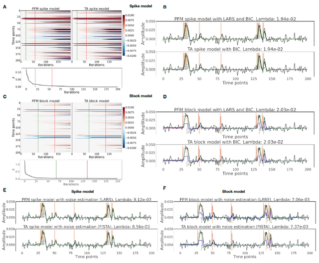
Figure 3: (A) Heatmap of the regularization paths of the activity-inducing signals (spike model) estimated with PFM and TA as a function of λ for the simulated data with SNR = 3 dB (x-axis: increasing number of iterations or λ as given by LARS; y-axis: time; color: amplitude). Vertical lines denote iterations corresponding to the BIC (dashed line) and MAD (dotted line) selection of λ. (B) Estimated activity-inducing (blue) and activity-related (green) signals with a selection of λ based on the BIC. Orange and red lines depict the ground truth. (C) Heatmap of the regularization paths of the innovation signals (block model) estimated with PFM and TA as a function of λ for the simulated data with SNR = 3 dB. (D) Estimated innovation (blue), activity-inducing (darker blue), and activity-related (green) signals with a selection of λ based on the BIC. (E) Activity-inducing and activity-related (fit, x) signals estimated with PFM (top) and TA (bottom) when λ is selected based on the MAD method with the spike model, and (F) with the block model for the simulated data with SNR = 3 dB.
noise for TA vs. finding the LARS residual that is closest to the MAD estimate of the noise), 319 higher RSSD values can be observed with the largest differences occurring in gray matter voxels. 320 These areas also correspond to low values of λ (see Figure S4) and MAD estimates of the noise 321 (see Figure S5), while the highest values are visible in regions with signal droupouts, ventricles, 322 and white matter. These differences that arise from the differing methods to find the optimal
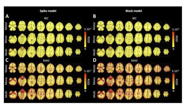
Figure 4: Square root of the sum of squared differences (RSSD) between the estimates obtained with PFM and TA for (A) spike model (activity-inducing signal) and BIC selection of λ, (B) block model (innovation signal) and BIC selection, (C) spike model (activity-inducing signal) and MAD selection, (D) block model (innovation signal) and MAD selection. RSSD maps are shown for the three experimental fMRI datasets: the motor task (Motor), the monoband resting-state (Mono), and the multiband resting-state (Multi) datasets.
regularization parameter based on the MAD estimate of the noise can be clearly seen in the root sum of squares (RSS) of the estimates of the two methods (Figure S6). These differences are also observable in the ATS calculated from estimates obtained with the MAD selection as shown in Figure S9. However, the identical regularization paths shown in Figure S7 demonstrate that both methods perform equivalently on experimental data (see estimates of innovation signal obtained with an identical selection of λ in Figure S8). Hence, the higher RSSD values originate from the different methods to find the optimal regularization parameter based on the MAD estimate of the noise that yield differnt solutions as shown by the dashed vertical lines in Figure S7.
Figure 5 depicts the results of the analysis of the Motor dataset with the PFM and TA algorithms using the BIC selection of λ (see Figure S9 for results with MAD selection), as well as a conventional GLM approach. The Activation Time Series (top left), calculated as the sum of squares of all voxel amplitudes (positive vs. negative) for a given moment in time, obtained with PFM and TA show nearly identical patterns. These ATS help to summarize the four dimensional information available in the results across the spatial domain and identify instances of significant BOLD activity. The second to sixth rows show the voxel timeseries and the corresponding activity-related, activity inducing and innovation signals obtained with PFM using the BIC criterion of representative voxels in the regions activated in each of the motor tasks. The TA-estimated time-series are not shown because they were virtually identical. The maps shown on the right correspond to statistical parametric maps obtained with the GLM for each motor condition (p < 0.001) as well as the maps of the PFM and TA estimates at the onsets of individual motor events (indicated with arrows in the timecourses). The estimated activity-related, activity-inducing and innovation signals clearly reveal the activity patterns of each condition in the task, as they exhibit a BOLD response locked to the onset and duration of the conditions. Overall, activity maps of the innovation signal obtained with PFM and TA highly resemble those obtained with a GLM for individual events, with small differences arising from the distinct specificity of the GLM and deconvolution analyses. Notice that the differences observed with the different approaches to select λ based on the MAD estimate shown in Figure 4 are reflected on the ATS shown in Figure S9 as well.
As an illustration of the insights that deconvolution methods can provide in the analysis of resting-state data, Figure 6 depicts the average activity-inducing and innovation maps of common resting-state networks obtained from thresholding and averaging the activity-inducing and innovation signals, respectively, estimated from the resting-state multiband data using PFM with a selection of λ based on the BIC. The average activity-inducing maps obtained via deconvolution show spatial patterns of the default mode network (DMN), dorsal attention network (DAN), and visual network (VIS) that highly resemble the maps obtained with conventional seed correlation analysis using Pearson’s correlation, and the average maps of extreme points of the signal (i.e., with no deconvolution). With deconvolution, the average activity-inducing maps seem to depict more accurate spatial delineation (i.e., less smoothness) than those obtained from the original data, while maintaining the structure of the networks. The BIC-informed selection of λ yields spatial patterns of average activity-inducing and innovation maps that are more sparse than those obtained with a selection of λ based on the MAD estimate (see Figure S10). Furthermore, the spatial patterns of the average innovation maps based on the innovation signals using the block model yield complementary information to those obtained with the activity-inducing signal since iCAPs allow to reveal regions with synchronous innovations, i.e., with the same upregulating and downregulating events. For instance, it is interesting to observe that the structure of the visual network nearly disappears in its corresponding average innovation maps, suggesting the existence of different temporal neuronal patterns across voxels in the primary and secondary visual cortices.
5. Discussion and conclusion
Hemodynamic deconvolution can be formulated using a synthesis- and analysis-based approach as proposed by PFM and TA, respectively. This work demonstrates that the theoretical equivalence of both approaches is confirmed in practice given virtually identical results when the same HRF model and equivalent regularization parameters are employed. Hence, we argue that previously observed differences in performance can be explained by specific settings, such as the HRF model and selection of the regularization parameter (as shown in Figures 4,S6 and S7), convergence thresholds, as well as the addition of a spatial regularization term in the spatiotemporal TA formulation (Karahanoğlu et al., 2013). For instance, the use of PFM with the spike model in (Tan et al., 2017) was seen not to be ideal due to the prolonged trials in the paradigm, which better fit the block model as described here (7). However, given the equivalence of the temporal deconvolution, incorporating extra spatial or temporal regularization terms in the optimization problem should not modify this equivalence providing convex operators are employed. For a convex optimization problem, with a unique global solution, iterative shrinkage thresholding procedures alternating between the different regularization terms guarantee convergence; e.g., the generalized forward-backward splitting (Raguet et al., 2013) algorithm originally employed for TA. Our findings are also in line with the equivalence of analysis and synthesis methods in under-determined cases (N ≤ V) demonstrated in
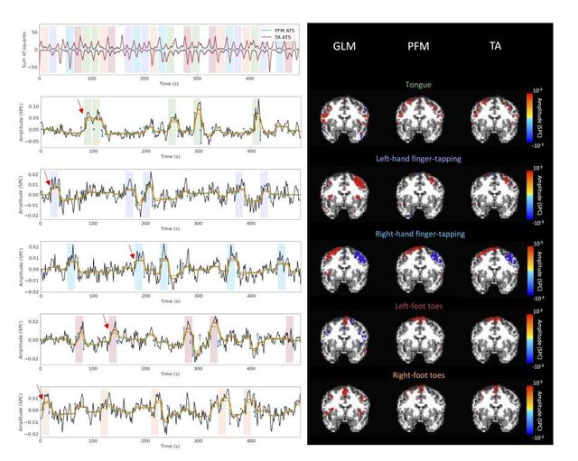
Figure 5: Activity maps of the motor task using a selection of λ based on the BIC estimate. Row 1: Activation time-series (ATS) of the innovation signals estimated by PFM (in blue) or TA (in red) calculated as the sum of squares of all voxels at every timepoint. Positive-valued and negative-valued contributions were separated into two distinct time-courses. Color-bands indicate the onset and duration of each condition in the task (green: tongue motion, purple: left-hand finger-tapping, blue: right-hand finger-tapping, red: left-foot toes motion, orange: right-foot toes motion). Rows 2–6: time-series of a representative voxel for each task with the PFM-estimated innovation (blue), PFM-estimated activity-inducing (green), and activity-related (i.e., fitted, orange) signals, with their corresponding GLM, PFM, and TA maps on the right (representative voxels indicated with green arrows). Amplitudes are given in signal percentage change (SPC). The maps shown on the right are sampled at the time-points labeled with the red arrows and display the innovation signals at these moments across the whole brain.
(Elad et al., 2007) and (Ortelli and van de Geer, 2019). Still, we have shown that a slight difference in the selection of the regularization parameter can lead to small differences in the estimated signals when employing the block model with the MAD selection of λ. However, since their regularization paths are equivalent, the algorithms can easily be forced to converge to the ame selection of λ, thus resulting in identical estimated signals.
Nevertheless, the different formulations of analysis and synthesis deconvolution models bring
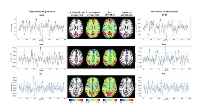
Figure 6: Average activity-inducing (left) and innovation (right) maps obtained from PFM-estimated activity-inducing and innovation signals, respectively, using a BIC-based selection of λ. Time-points selected with a 95th percentile threshold (horizontal lines) are shown over the average time-series (blue) in the seed region (white cross) and the deconvolved signals, i.e., activity inducing (left) and innovation (right) signals (orange). Average maps of extreme points and seed correlation maps are illustrated in the center.
along different kinds of flexibility. One notable advantage of PFM is that it can readily incorporate any HRF as part of the synthesis operator (Elad et al., 2007), only requiring the sampled HRF at the desired temporal resolution, which is typically equal to the TR of the acquisition. Conversely, TA relies upon the specification of the discrete differential operator that inverts the HRF, which needs to be derived either by the inverse solution of the sampled HRF impulse response, or by discretizing a continuous-domain differential operator motivated by a biophysical model. The more versatile structure of PFM allows for instance an elegant extension of the algorithm to multi-echo fMRI data (Caballero-Gaudes et al., 2019) where multiple measurements relate to a common underlying signal. Therefore, the one-to-many synthesis scenario (i.e., from activity-inducing to several activity related signals) is more cumbersome to express using TA; i.e., a set of differential operators should be defined and the differences between their outputs constrained. Conversely, the one-to-many analysis scenario (i.e., from the measurements to several regularizing signals) is more convenient to be expressed by TA; e.g., combining spike and block regularizers. While the specification of the differential operator in TA only indirectly controls the HRF, the use of the derivative operator to enforce the block model, instead of the integrator in PFM, impacts positively the stability and rate of the convergence of the optimization algorithms. Moreover, analysis formulations can be more suitable for online applications that are still to be explored in fMRI data, but are employed for calcium imaging deconvolution (Friedrich et al., 2017; Jewell et al., 2019), and which have been applied for offline calcium deconvolution (Farouj et al., 2020).
Deconvolution techniques can be used before more downstream analysis of brain activity in terms of functional network organization as they estimate interactions between voxels or brain regions that occur at the activity-inducing level, and are thus less affected by the slowness of the hemodynamic response compared to when the BOLD signals are analyzed directly. In addition, deconvolution approaches hold a close parallelism to recent methodologies aiming to understand the dynamics of neuronal activations and interactions at short temporal resolution and that focus on extreme events of the fMRI signal (Lindquist et al., 2007). As an illustration, Figure 6 shows that the innovation- or activity-inducing CAPs computed from deconvolved events in a single resting-state fMRI dataset closely resemble the conventional CAPs computed directly from extreme events of the fMRI signal (Liu and Duyn, 2013; Liu et al., 2013 2018; Cifre et al., 2020a,b; Zhang et al., 2020; Tagliazucchi et al., 2011, 2012, 2016; Rolls et al., 2021). Similarly, we hypothesize that these extreme events will also show a close resemblance to intrinsic ignition events (Deco and Kringelbach, 2017; Deco et al., 2017). As shown in the maps, deconvolution approaches can offer a more straightforward interpretability of the activation events and resulting functional connectivity patterns. Here, CAPs were computed as the average of spatial maps corresponding to the events of a single dataset. Beyond simple averaging, clustering algorithms (e.g., K-means and consensus clustering) can be employed to discern multiple CAPs or iCAPs at the whole-brain level for a large number of subjects. Previous findings based on iCAPs have for instance revealed organizational principles of brain function during rest (Karahanoğlu and Ville, 2015) and sleep (Tarun et al., 2021) in healthy controls, next to alterations in 22q11ds (Zoeller et al., 2019) and multiple sclerosis (Bommarito et al., in press). Next to CAPs-inspired approaches, dynamic functional connectivity has recently been investigated with the use of co-fluctuations and edge-centric techniques (Faskowitz et al., 2020; Esfahlani et al., 2020; Jo et al., 2021; Sporns et al., 2021; van Oort et al., 2018). The activation time series shown in Figure 5 aim to provide equivalent information to the root of sum of squares timecourses used in edge-centric approaches, where timecourses with peaks delineate instances of significant brain activity. Future work could address which type of information is redundant or distinct across these frameworks. In summary, these examples illustrate that deconvolution techniques can be employed prior to other computational approaches and could serve as an effective way of denoising the fMRI data. We foresee an increase in the number of studies that take advantage of the potential benefits of using deconvolution methods prior to functional connectivity analyses.
In sum, hemodynamic deconvolution approaches using sparsity-driven regularization are valuable tools to complete the fMRI processing pipeline. Although the two approaches examined in detail here provide alternative representations of the BOLD signals in terms of innovation and activity-inducing signals, their current implementations have certain limitations, calling for further developments or more elaborate models, where some of them have been initially addressed in the literature. One relevant focus is to account for the variability in HRF that can be observed in different regions of the brain. First, variability in the temporal characteristics of the HRF can arise from differences in stimulus intensity and patterns, as well as with short inter-event intervals like in fast cognitive processes or experimental designs (Yeşilyurt et al., 2008; Sadaghiani et al., 2009; Chen et al., 2021; Polimeni and Lewis, 2021). Similarly, the HRF shape at rest might differ from the canonical HRF commonly used for task-based fMRI data analysis. A wide variety of HRF patterns could be elicited across the whole brain and possible detected with sufficiently large signal-to-noise ratio, e.g., (Gonzalez-Castillo et al., 2012) showed two gamma-shaped responses at the onset and the end of the evoked trial, respectively. This unique HRF shape would be deconvolved as two separate events with the conventional deconvolution techniques. The impact of HRF variability could be reduced using structured regularization terms along with multiple basis functions (Gaudes et al., 2012) or procedures that estimate the HRF shape in an adaptive fashion in both analysis (Farouj et al., 2019) and synthesis formulations (Cherkaoui et al., 2020a).
Another avenue of research consists in leveraging spatial information by adopting multivariate deconvolution approaches that operate at the whole-brain level, instead of working voxelwise and beyond regional regularization terms (e.g. as proposed in Karahanoğlu et al. 2013). Operating at the whole-brain level would open the way for methods that consider shared neuronal activity using mixed norm regularization terms (Uruñuela-Tremiño et al., 2019) or can capture long-range neuronal cofluctuations using low rank decompositions (Cherkaoui et al., 2020a). For example, multivariate deconvolution approaches could yield better localized activity patterns while reducing the effect of global fluctuations such as respiratory artifacts, which cannot be modelled at the voxel level (Urunñuela et al., 2021).
Similar to solving other inverse problems by means of regularized estimators, the selection of the regularization parameter is critical to correctly estimate the neuronal-related signal. Hence, methods that take advantage of a more robust selection of the regularization parameter could considerably yield more reliable estimates of the neuronal-related signal. For instance, the stability selection (Meinshausen and Bühlmann, 2010; Uruñuela et al., 2020) procedure could be included to the deconvolution problem to ensure that the estimated coefficients are obtained with high probability. Furthermore, an important issue of regularized estimation is that the estimates are biased with respect to the true value. In that sense, the use of non-convex 𝓵p,q-norm regularization terms (e.g., p < 1) can reduce this bias while maintaining the sparsity constraint, at the cost of potentially converging to a local minima of the regularized estimation problem. In practice, these approaches could avoid the optional debiasing step that overcomes the shrinkage of the estimates and obtain a more accurate and less biased fit of the fMRI signal (Gaudes et al., 2013; Caballero-Gaudes et al., 2019). Finally, cutting-edge developments on physics-informed deep learning techniques for inverse problems (Akçakaya et al., 2021; Monga et al., 2021; Ongie et al., 2020; Cherkaoui et al., 2020b) could be transferred for deconvolution by considering the biophysical model of the hemodynamic system and could potentially offer algorithms with reduced computational time and more flexibility.
6. Code and data availability
The code and materials used in this work can be found in the following GitHub repository: https://github.com/eurunuela/pfm_vs_ta. We encourage the reader to explore the parameters (e.g., SNR, varying HRF options and mismatch between algorithms, TR, number of events, onsets, and durations) in the provided Jupyter notebooks. Likewise, the data used to produce the figures can be found in https://osf.io/f3ryg/.
7. Acknowledgements
We thank Stefano Moia and Vicente Ferrer for data availability, and Younes Farouj for valuable comments on the manuscript. This research was funded by the Spanish Ministry of Economy and Competitiveness (RYC–2017–21845), the Basque Government (BERC 2018–2021, PIB_2019_104, PRE_2020_2_0227), and the Spanish Ministry of Science, Innovation and Universities (PID2019–105520GB–100), and the Swiss National Science Foundation (grant 205321_163376).
8. CRediT
Eneko Uruñuela: Conceptualisation, Methodology, Software, Formal Analysis, Investigation, Data Curation, Writing (OD), Writing (RE), Visualisation, Funding acquisition. Thomas A. W. Bolton: Conceptualisation, Methodology, Writing (RE). Dimitri Van de Ville: Conceptualisation, Methodology, Writing (RE). César Caballero-Gaudes: Conceptualisation, Methodology, Software, Formal Analysis, Investigation, Data Curation, Writing (OD), Writing (RE), Visualisation, Funding acquisition.
References
Akçakaya, M., Yaman, B., Chung, H., Ye, J. C., 2021. Unsupervised deep learning methods for biological image reconstruction arXiv:2105.08040.
Allan, T. W., Francis, S. T., Caballero-Gaudes, C., Morris, P. G., Liddle, E. B., Liddle, P. F., … Gowland, P. A. (2015). Functional Connectivity in MRI Is Driven by Spontaneous BOLD Events. PLOS ONE, 10(4), e0124577. https://doi.org/10.1371/JOURNAL.PONE.0124577
Andersson, J. L., Skare, S., Ashburner, J., 2003. How to correct susceptibility distortions in spinecho echo-planar images: application to diffusion tensor imaging. NeuroImage 20, 870–888. doi:10.1016/s1053–8119(03)00336–7.
Aslan, S., Cemgil, A. T., Akin, A., 2016. Joint state and parameter estimation of the hemodynamic model by particle smoother expectation maximization method. Journal of Neural Engineering 13, 046010. doi:10.1088/1741–2560/13/4/046010.
Beck, A., & Teboulle, M. (2009). A Fast Iterative Shrinkage-Thresholding Algorithm for Linear Inverse Problems. SIAM Journal on Imaging Sciences, 2(1), 183–202. https://doi.org/10.1137/080716542
Behzadi, Y., Restom, K., Liau, J., & Liu, T. T. (2007). A component based noise correction method (CompCor) for BOLD and perfusion based fMRI. NeuroImage, 37(1), 90–101. https://doi.org/10.1016/J.NEUROIMAGE.2007.04.042
Birn, R. M., Diamond, J. B., Smith, M. A., & Bandettini, P. A. (2006). Separating respiratory-variation-related fluctuations from neuronal-activity-related fluctuations in fMRI. NeuroImage, 31(4), 1536–1548. https://doi.org/10.1016/J.NEUROIMAGE.2006.02.048
Bolton, T. A. W., Morgenroth, E., Preti, M. G., & Van De Ville, D. (2020). Tapping into Multi-Faceted Human Behavior and Psychopathology Using fMRI Brain Dynamics. Trends in Neurosciences. https://doi.org/10.1016/J.TINS.2020.06.005
Bommarito, G., Tarun, A., Farouj, Y., Preti, M. G., Petracca, M., Droby, A., Mendili, M. M. E., Inglese, M., Ville, D. V. D., 2020. Altered anterior default mode network dynamics in progressive multiple sclerosis. medRxiv doi:10.1101/2020.11.26.20238923.
Bommarito, G., Tarun, A., Farouj, Y., Preti, M. G., Petracca, M., Droby, A., Mounir El Mendili, M., Inglese, M., Van De Ville, D., in press. Altered anterior default mode network dynamics in progressive multiple sclerosis. Multiple Sclerosis Journal doi:10.1177/13524585211018116.
Boynton, G. M., Engel, S. A., Glover, G. H., & Heeger, D. J. (1996). Linear Systems Analysis of Functional Magnetic Resonance Imaging in Human V1. The Journal of Neuroscience, 16(13), 4207–4221. https://doi.org/10.1523/JNEUROSCI.16-13-04207.1996
Bruckstein, A. M., Donoho, D. L., & Elad, M. (2009). From Sparse Solutions of Systems of Equations to Sparse Modeling of Signals and Images. SIAM Review, 51(1), 34–81. https://doi.org/10.1137/060657704
Bush, K., Cisler, J., 2013. Decoding neural events from fMRI BOLD signal: A comparison of existing approaches and development of a new algorithm. Magnetic Resonance Imaging 31, 976–989. doi:10.1016/j.mri.2013.03.015.
Bush, K., Zhou, S., Cisler, J., Bian, J., Hazaroglu, O., Gillispie, K., Yoshigoe, K., Kilts, C., 2015. A deconvolution-based approach to identifying large-scale effective connectivity. Magnetic Resonance Imaging 33, 1290–1298. doi:10.1016/j.mri.2015.07.015.
Buxton, R. B., Wong, E. C., Frank, L. R., 1998. Dynamics of blood flow and oxygenation changes during brain activation: the balloon model. Magnetic resonance in medicine 39, 855–864.
Caballero-Gaudes, C., Moia, S., Panwar, P., Bandettini, P. A., Gonzalez-Castillo, J., 2019. A deconvolution algorithm for multi-echo functional MRI: Multi-echo sparse paradigm free mapping. NeuroImage 202, 116081. doi:10.1016/j.neuroimage.2019.116081.
Casanova, R., Ryali, S., Serences, J., Yang, L., Kraft, R., Laurienti, P. J., Maldjian, J. A., 2008. The impact of temporal regularization on estimates of the BOLD hemodynamic response function: A comparative analysis. NeuroImage 40, 1606–1618. doi:10.1016/j.neuroimage.2008.01.011.
Chambolle, A., 2004. An algorithm for total variation minimization and applications. Journal of Mathematical imaging and vision 20, 89–97.
Chen, J. E., Glover, G. H., Fultz, N. E., Rosen, B. R., Polimeni, J. R., Lewis, L. D., 2021. Investigating mechanisms of fast BOLD responses: The effects of stimulus intensity and of spatial heterogeneity of hemodynamics. NeuroImage 245, 118658. doi:10.1016/j.neuroimage.2021.118658.
Chen, S. S., Donoho, D. L., Saunders, M. A., 2001. Atomic decomposition by basis pursuit. SIAM review 43, 129–159.
Cherkaoui, H., Moreau, T., Halimi, A., & Ciuciu, P. (2019). Sparsity-based Blind Deconvolution of Neural Activation Signal in FMRI. Institute of Electrical and Electronics Engineers (IEEE). https://doi.org/10.1109/ICASSP.2019.8683358
Cherkaoui, H., Moreau, T., Halimi, A., Leroy, C., Ciuciu, P., 2020a. Multivariate semi-blind deconvolution of fMRI time series. URL: https://hal.archives-ouvertes.fr/hal–03005584. working paper or preprint.
Cherkaoui, H., Sulam, J., Moreau, T., 2020b. Learning to solve TV regularised problems with unrolled algorithms 33, 11513–11524. URL: https://proceedings.neurips.cc/paper/2020/file/84fec9a8e45846340fdf5c7c9f7ed66c-Paper.pdf.
Cifre, I., Flores, M. T. M., Ochab, J. K., Chialvo, D. R., 2020a. Revisiting non-linear functional brain co-activations: directed, dynamic and delayed. arXiv:2007.15728.
Cifre, I., Zarepour, M., Horovitz, S. G., Cannas, S. A., & Chialvo, D. R. (2020). Further results on why a point process is effective for estimating correlation between brain regions. Papers in Physics, 12, 120003. https://doi.org/10.4279/PIP.120003
Ciuciu, P., Poline, J. B., Marrelec, G., Idier, J., Pallier, C., Benali, H., 2003. Unsupervised robust nonparametric estimation of the hemodynamic response function for any fmri experiment. IEEE transactions on medical imaging 22, 1235–1251. doi:10.1109/TMI.2003.817759.
Cohen, M. S. (1997). Parametric Analysis of fMRI Data Using Linear Systems Methods. NeuroImage, 6(2), 93–103. https://doi.org/10.1006/NIMG.1997.0278
Costantini, I., Deriche, R., & Deslauriers-Gauthier, S. (2022). An Anisotropic 4D Filtering Approach to Recover Brain Activation From Paradigm-Free Functional MRI Data. Frontiers in Neuroimaging, 1, 815423. https://doi.org/10.3389/FNIMG.2022.815423
Cox, R. W. (1996). AFNI: Software for Analysis and Visualization of Functional Magnetic Resonance Neuroimages. Computers and Biomedical Research, 29(3), 162–173. https://doi.org/10.1006/CBMR.1996.0014
Deco, G., & Kringelbach, M. L. (2017). Hierarchy of Information Processing in the Brain: A Novel ‘Intrinsic Ignition’ Framework. Neuron, 94(5), 961–968. https://doi.org/10.1016/J.NEURON.2017.03.028
Deco, G., Tagliazucchi, E., Laufs, H., Sanjuán, A., Kringelbach, M. L., 2017. Novel intrinsic ignition method measuring local-global integration characterizes wakefulness and deep sleep. eNeuro 4. doi:10.1523/ENEURO.0106–17.2017.
Di, X., & Biswal, B. B. (2013). Modulatory Interactions of Resting-State Brain Functional Connectivity. PLoS ONE, 8(8), e71163. https://doi.org/10.1371/JOURNAL.PONE.0071163
Di (??????), X., & Biswal, B. B. (2015). Characterizations of resting-state modulatory interactions in the human brain. Journal of Neurophysiology, 114(5), 2785–2796. https://doi.org/10.1152/JN.00893.2014
Di, X., & Biswal, B. B. (2019). Toward Task Connectomics: Examining Whole-Brain Task Modulated Connectivity in Different Task Domains. Cerebral Cortex, 29(4), 1572–1583. https://doi.org/10.1093/CERCOR/BHY055
Tibshirani, R., Johnstone, I., Hastie, T., & Efron, B. (2004). Least angle regression. The Annals of Statistics, 32(2), 407–499. https://doi.org/10.1214/009053604000000067
Elad, M., Milanfar, P., & Rubinstein, R. (2007). Analysis versus synthesis in signal priors. Inverse Problems, 23(3), 947–968. https://doi.org/10.1088/0266-5611/23/3/007
Zamani Esfahlani, F., Jo, Y., Faskowitz, J., Byrge, L., Kennedy, D. P., Sporns, O., & Betzel, R. F. (2020). High-amplitude cofluctuations in cortical activity drive functional connectivity. Proceedings of the National Academy of Sciences, 117(45), 28393–28401. https://doi.org/10.1073/PNAS.2005531117
Farouj, Y., Karahanoglu, F. I., Ville, D. V. D., 2019. Bold signal deconvolution under uncertain hÆmodynamics: A semi-blind approach, in: 2019 IEEE 16th International Symposium on Biomedical Imaging (ISBI 2019), IEEE. IEEE. pp. 1792–1796. doi:10.1109/isbi.2019.8759248.
Farouj, Y., Karahanoglu, F. I., Ville, D. V. D., 2020. Deconvolution of sustained neural activity from large-scale calcium imaging data 39, 1094–1103. doi:10.1109/tmi.2019.2942765.
Faskowitz, J., Esfahlani, F. Z., Jo, Y., Sporns, O., & Betzel, R. F. (2020). Edge-centric functional network representations of human cerebral cortex reveal overlapping system-level architecture. Nature Neuroscience. https://doi.org/10.1038/S41593-020-00719-Y
Feinberg, D. A., Moeller, S., Smith, S. M., Auerbach, E., Ramanna, S., Glasser, M. F., … Yacoub, E. (2010). Multiplexed Echo Planar Imaging for Sub-Second Whole Brain FMRI and Fast Diffusion Imaging. PLoS ONE, 5(12), e15710. https://doi.org/10.1371/JOURNAL.PONE.0015710
Freitas, L. G. A., Bolton, T. A. W., Krikler, B. E., Jochaut, D., Giraud, A.-L., Hüppi, P. S., & Van De Ville, D. (2020). Time-resolved effective connectivity in task fMRI: Psychophysiological interactions of Co-Activation patterns. NeuroImage, 212, 116635. https://doi.org/10.1016/J.NEUROIMAGE.2020.116635
Friedrich, J., Zhou, P., & Paninski, L. (2017). Fast online deconvolution of calcium imaging data. PLOS Computational Biology, 13(3), e1005423. https://doi.org/10.1371/JOURNAL.PCBI.1005423
Friston, K. J., Fletcher, P., Josephs, O., Holmes, A., Rugg, M. D., & Turner, R. (1998). Event-Related fMRI: Characterizing Differential Responses. NeuroImage, 7(1), 30–40. https://doi.org/10.1006/NIMG.1997.0306
Friston, K. J., Trujillo-Barreto, N., & Daunizeau, J. (2008). DEM: A variational treatment of dynamic systems. NeuroImage, 41(3), 849–885. https://doi.org/10.1016/J.NEUROIMAGE.2008.02.054
Friston, K. J., Jezzard, P., & Turner, R. (1994). Analysis of functional MRI time-series. Human Brain Mapping, 1(2), 153–171. https://doi.org/10.1002/HBM.460010207
Friston, K. J., Mechelli, A., Turner, R., Price, C. J., 2000. Nonlinear responses in fmri: the balloon model, volterra kernels, and other hemodynamics. NeuroImage 12, 466–477.
Gaudes, C. C., Karahanoglu, F. I., Lazeyras, F., Ville, D. V. D., 2012. Structured sparse deconvolution for paradigm free mapping of functional MRI data, in: 2012 9th IEEE International Symposium on Biomedical Imaging (ISBI), IEEE. IEEE. pp. 322–325. doi:10.1109/isbi.2012.6235549.
Gaudes, C. C., Petridou, N., Dryden, I. L., Bai, L., Francis, S. T., & Gowland, P. A. (2011). Detection and characterization of single-trial fMRI bold responses: Paradigm free mapping. Human Brain Mapping, 32(9), 1400–1418. https://doi.org/10.1002/HBM.21116
Caballero Gaudes, C., Petridou, N., Francis, S. T., Dryden, I. L., & Gowland, P. A. (2011). Paradigm free mapping with sparse regression automatically detects single-trial functional magnetic resonance imaging blood oxygenation level dependent responses. Human Brain Mapping, n/a-n/a. https://doi.org/10.1002/HBM.21452
Gaudes, C. C., Van De Ville, D., Petridou, N., Lazeyras, F., Gowland, P., 2011. Paradigm-free mapping with morphological component analysis: Getting most out of fmri data, in: Wavelets and Sparsity XIV, International Society for Optics and Photonics. p. 81381K.
Gerchen, M. F., Bernal-Casas, D., & Kirsch, P. (2014). Analyzing task-dependent brain network changes by whole-brain psychophysiological interactions: A comparison to conventional analysis. Human Brain Mapping, 35(10), 5071–5082. https://doi.org/10.1002/HBM.22532
Gitelman, D. R., Penny, W. D., Ashburner, J., Friston, K. J., 2003. Modeling regional and psychophysiologic interactions in fMRI: the importance of hemodynamic deconvolution. NeuroImage 19, 200–207. doi:10.1016/s1053–8119(03)00058–2.
Glasser, M. F., Smith, S. M., Marcus, D. S., Andersson, J. L. R., Auerbach, E. J., Behrens, T. E. J., … Van Essen, D. C. (2016). The Human Connectome Project’s neuroimaging approach. Nature Neuroscience, 19(9), 1175–1187. https://doi.org/10.1038/NN.4361
Glover, G. H. (1999). Deconvolution of Impulse Response in Event-Related BOLD fMRI1. NeuroImage, 9(4), 416–429. https://doi.org/10.1006/NIMG.1998.0419
Gonzalez-Castillo, J., Caballero-Gaudes, C., Topolski, N., Handwerker, D. A., Pereira, F., & Bandettini, P. A. (2019). Imaging the spontaneous flow of thought: Distinct periods of cognition contribute to dynamic functional connectivity during rest. NeuroImage, 202, 116129. https://doi.org/10.1016/J.NEUROIMAGE.2019.116129
Gonzalez-Castillo, J., Saad, Z. S., Handwerker, D. A., Inati, S. J., Brenowitz, N., & Bandettini, P. A. (2012). Whole-brain, time-locked activation with simple tasks revealed using massive averaging and model-free analysis. Proceedings of the National Academy of Sciences, 109(14), 5487–5492. https://doi.org/10.1073/PNAS.1121049109
Goutte, C., Nielsen, F. A., Hansen, L. K., 2000. Modeling the haemodynamic response in fmri using smooth fir filters. IEEE transactions on medical imaging 19, 1188–1201. doi:10.1109/42.897811.
Havlicek, M., Friston, K. J., Jan, J., Brazdil, M., & Calhoun, V. D. (2011). Dynamic modeling of neuronal responses in fMRI using cubature Kalman filtering. NeuroImage, 56(4), 2109–2128. https://doi.org/10.1016/J.NEUROIMAGE.2011.03.005
Henson, R., Friston, K., 2007. Chapter 14 - convolution models for fmri, in: Friston, K., Ashburner, J., Kiebel, S., Nichols, T., Penny, W. (Eds.), Statistical Parametric Mapping. Academic Press, London, pp. 178–192. URL: https://www.sciencedirect.com/science/article/pii/B9780123725608500140, doi:https://doi.org/10.1016/B978–012372560–8/50014–0.
Hernandez-Garcia, L., Ulfarsson, M. O., 2011. Neuronal event detection in fMRI time series using iterative deconvolution techniques. Magnetic Resonance Imaging 29, 353–364. doi:10.1016/j.mri.2010.10.012.
H??tel, M., Antonelli, M., Melbourne, A., & Ourselin, S. (2021). Hemodynamic matrix factorization for functional magnetic resonance imaging. NeuroImage, 231, 117814. https://doi.org/10.1016/J.NEUROIMAGE.2021.117814
Hüitel, M., Melbourne, A., Ourselin, S., 2018. Neural activation estimation in brain networks during task and rest using BOLD-fMRI, in: Medical Image Computing and Computer Assisted Intervention—MICCAI 2018, Springer. Springer International Publishing. pp. 215–222. doi:10.1007/978–3–030–00931–1_25.
Jenkinson, M., Beckmann, C. F., Behrens, T. E. J., Woolrich, M. W., & Smith, S. M. (2012). FSL. NeuroImage, 62(2), 782–790. https://doi.org/10.1016/J.NEUROIMAGE.2011.09.015
Jenkinson, M., Smith, S., 2001. A global optimisation method for robust affine registration of brain images. Medical Image Analysis 5, 143–156. doi:10.1016/s1361–8415(01)00036–6.
Jewell, S. W., Hocking, T. D., Fearnhead, P., & Witten, D. M. (2019). Fast nonconvex deconvolution of calcium imaging data. Biostatistics. https://doi.org/10.1093/BIOSTATISTICS/KXY083
Jo, Y., Faskowitz, J., Esfahlani, F. Z., Sporns, O., & Betzel, R. F. (2021). Subject identification using edge-centric functional connectivity. NeuroImage, 238, 118204. https://doi.org/10.1016/J.NEUROIMAGE.2021.118204
Karahanoglu, F. I., Bayram, ??lker, & Van De Ville, D. (2011). A Signal Processing Approach to Generalized 1-D Total Variation. IEEE Transactions on Signal Processing, 59(11), 5265–5274. https://doi.org/10.1109/TSP.2011.2164399
Karahano??lu, F. I., Caballero-Gaudes, C., Lazeyras, F., & Van De Ville, D. (2013). Total activation: fMRI deconvolution through spatio-temporal regularization. NeuroImage, 73, 121–134. https://doi.org/10.1016/J.NEUROIMAGE.2013.01.067
Karahanoglu, F. I., Grouiller, F., Gaudes, C. C., Seeck, M., Vulliemoz, S., Ville, D. V. D., 2013. Spatial mapping of interictal epileptic discharges in fMRI with total activation, in: 2013 IEEE 10th International Symposium on Biomedical Imaging, Ieee. IEEE. pp. 1500–1503. doi:10.1109/isbi.2013.6556819.
Karahanoğlu, F. I., & Van De Ville, D. (2015). Transient brain activity disentangles fMRI resting-state dynamics in terms of spatially and temporally overlapping networks. Nature Communications, 6(1). https://doi.org/10.1038/NCOMMS8751
Karahanoğlu, F. I., & Van De Ville, D. (2017). Dynamics of large-scale fMRI networks: Deconstruct brain activity to build better models of brain function. Current Opinion in Biomedical Engineering, 3, 28–36. https://doi.org/10.1016/J.COBME.2017.09.008
Keilholz, S., Caballero-Gaudes, C., Bandettini, P., Deco, G., & Calhoun, V. (2017). Time-Resolved Resting-State Functional Magnetic Resonance Imaging Analysis: Current Status, Challenges, and New Directions. Brain Connectivity, 7(8), 465–481. https://doi.org/10.1089/BRAIN.2017.0543
Khalidov, I., Fadili, J., Lazeyras, F., Ville, D. V. D., Unser, M., 2011. Activelets: Wavelets for sparse representation of hemodynamic responses. Signal Processing 91, 2810–2821. doi:10.1016/j.sigpro.2011.03.008.
Kinany, N., Pirondini, E., Micera, S., & Van De Ville, D. (2020). Dynamic Functional Connectivity of Resting-State Spinal Cord fMRI Reveals Fine-Grained Intrinsic Architecture. Neuron, 108(3), 424-435.e4. https://doi.org/10.1016/J.NEURON.2020.07.024
Lindquist, M. A., Waugh, C., & Wager, T. D. (2007). Modeling state-related fMRI activity using change-point theory. NeuroImage, 35(3), 1125–1141. https://doi.org/10.1016/J.NEUROIMAGE.2007.01.004
Liu, X., Chang, C., & Duyn, J. H. (2013). Decomposition of spontaneous brain activity into distinct fMRI co-activation patterns. Frontiers in Systems Neuroscience, 7. https://doi.org/10.3389/FNSYS.2013.00101
Liu, X., & Duyn, J. H. (2013). Time-varying functional network information extracted from brief instances of spontaneous brain activity. Proceedings of the National Academy of Sciences, 110(11), 4392–4397. https://doi.org/10.1073/PNAS.1216856110
Liu, X., Zhang, N., Chang, C., & Duyn, J. H. (2018). Co-activation patterns in resting-state fMRI signals. NeuroImage, 180, 485–494. https://doi.org/10.1016/J.NEUROIMAGE.2018.01.041
Lopes, R., Lina, J. M., Fahoum, F., & Gotman, J. (2012). Detection of epileptic activity in fMRI without recording the EEG. NeuroImage, 60(3), 1867–1879. https://doi.org/10.1016/J.NEUROIMAGE.2011.12.083
Loula, J., Varoquaux, G., Thirion, B., 2018. Decoding fMRI activity in the time domain improves classification performance. NeuroImage 180, 203–210. doi:10.1016/j.neuroimage.2017.08.018.
Lurie, D. J., Kessler, D., Bassett, D. S., Betzel, R. F., Breakspear, M., Kheilholz, S., … Calhoun, V. D. (2020). Questions and controversies in the study of time-varying functional connectivity in resting fMRI. Network Neuroscience, 4(1), 30–69. https://doi.org/10.1162/NETN_A_00116
Madi, M. K., Karameh, F. N., 2017. Hybrid cubature kalman filtering for identifying nonlinear models from sampled recording: Estimation of neuronal dynamics. PLOS ONE 12, e0181513. doi:10.1371/journal.pone.0181513.
Marrelec, G., Benali, H., Ciuciu, P., Poline, J. B., 2002. Bayesian estimation of the hemodynamic response function in functional mri. AIP Conference Proceedings 617, 229–247. URL: https://aip.scitation.org/doi/abs/10.1063/1.1477050, doi:10.1063/1.1477050, arXiv:https://aip.scitation.org/doi/pdf/10.1063/1.1477050.
Meinshausen, N., & Bühlmann, P. (2010). Stability selection. Journal of the Royal Statistical Society: Series B (Statistical Methodology), 72(4), 417–473. https://doi.org/10.1111/J.1467-9868.2010.00740.X
Moeller, S., Yacoub, E., Olman, C. A., Auerbach, E., Strupp, J., Harel, N., & Uğurbil, K. (2010). Multiband multislice GE-EPI at 7 tesla, with 16-fold acceleration using partial parallel imaging with application to high spatial and temporal whole-brain fMRI. Magnetic Resonance in Medicine, 63(5), 1144–1153. https://doi.org/10.1002/MRM.22361
Monga, V., Li, Y., & Eldar, Y. C. (2021). Algorithm Unrolling: Interpretable, Efficient Deep Learning for Signal and Image Processing. IEEE Signal Processing Magazine, 38(2), 18–44. https://doi.org/10.1109/MSP.2020.3016905
Ongie, G., Jalal, A., Metzler, C. A., Baraniuk, R. G., Dimakis, A. G., & Willett, R. (2020). Deep Learning Techniques for Inverse Problems in Imaging. IEEE Journal on Selected Areas in Information Theory, 1(1), 39–56. https://doi.org/10.1109/JSAIT.2020.2991563
van Oort, E. S. B., Mennes, M., Navarro Schr??der, T., Kumar, V. J., Zaragoza Jimenez, N. I., Grodd, W., … Beckmann, C. F. (2018). Functional parcellation using time courses of instantaneous connectivity. NeuroImage, 170, 31–40. https://doi.org/10.1016/J.NEUROIMAGE.2017.07.027
Ortelli, F., van de Geer, S., 2019. Synthesis and analysis in total variation regularization. arXiv:1901.06418.
Patriat, R., Molloy, E. K., & Birn, R. M. (2015). Using Edge Voxel Information to Improve Motion Regression for rs-fMRI Connectivity Studies. Brain Connectivity, 5(9), 582–595. https://doi.org/10.1089/BRAIN.2014.0321
Penny, W., Ghahramani, Z., & Friston, K. (2005). Bilinear dynamical systems. Philosophical Transactions of the Royal Society B: Biological Sciences, 360(1457), 983–993. https://doi.org/10.1098/RSTB.2005.1642
Petridou, N., Gaudes, C. C., Dryden, I. L., Francis, S. T., & Gowland, P. A. (2012). Periods of rest in fMRI contain individual spontaneous events which are related to slowly fluctuating spontaneous activity. Human Brain Mapping, 34(6), 1319–1329. https://doi.org/10.1002/HBM.21513
Pidnebesna, A., Fajnerová, I., Horáček, J., Hlinka, J., 2019. Estimating sparse neuronal signal from hemodynamic response: the mixture components inference approach. bioRxiv doi:10.1101/2019.12.19.876508.
Polimeni, J. R., & Lewis, L. D. (2021). Imaging faster neural dynamics with fast fMRI: A need for updated models of the hemodynamic response. Progress in Neurobiology, 207, 102174. https://doi.org/10.1016/J.PNEUROBIO.2021.102174
Posse, S., Wiese, S., Gembris, D., Mathiak, K., Kessler, C., Grosse-Ruyken, M. L., Elghahwagi, B., Richards, T., Dager, S. R., Kiselev, V. G., 1999. Enhancement of BOLD-contrast sensitivity by single-shot multi-echo functional MR imaging. Magnetic Resonance in Medicine 42, 87–97. doi:10.1002/(sici)1522–2594(199907)42:1<87::aid-mrm13>3.0.co;2-o.
Preti, M. G., Bolton, T. A., & Van De Ville, D. (2017). The dynamic functional connectome: State-of-the-art and perspectives. NeuroImage, 160, 41–54. https://doi.org/10.1016/J.NEUROIMAGE.2016.12.061
Raguet, H., Fadili, J., & Peyré, G. (2013). A Generalized Forward-Backward Splitting. SIAM Journal on Imaging Sciences, 6(3), 1199–1226. https://doi.org/10.1137/120872802
Riera, J. J., Watanabe, J., Kazuki, I., Naoki, M., Aubert, E., Ozaki, T., & Kawashima, R. (2004). A state-space model of the hemodynamic approach: nonlinear filtering of BOLD signals. NeuroImage, 21(2), 547–567. https://doi.org/10.1016/J.NEUROIMAGE.2003.09.052
Rolls, E. T., Cheng, W., & Feng, J. (2021). Brain dynamics: Synchronous peaks, functional connectivity, and its temporal variability. Human Brain Mapping, 42(9), 2790–2801. https://doi.org/10.1002/HBM.25404
Ruiz-Euler, H. C., Marques, J. R. F., Kappen, H. J., 2018. Nonlinear deconvolution by sampling biophysically plausible hemodynamic models. arXiv:1803.08797.
Sadaghiani, S., U??urbil, K., & Uluda??, K. (2009). Neural activity-induced modulation of BOLD poststimulus undershoot independent of the positive signal. Magnetic Resonance Imaging, 27(8), 1030–1038. https://doi.org/10.1016/J.MRI.2009.04.003
Schwarz, G. (1978). Estimating the Dimension of a Model. The Annals of Statistics, 6(2), 461–464. https://doi.org/10.1214/AOS/1176344136
Setsompop, K., Gagoski, B. A., Polimeni, J. R., Witzel, T., Wedeen, V. J., & Wald, L. L. (2012). Blipped-controlled aliasing in parallel imaging for simultaneous multislice echo planar imaging with reduced g-factor penalty. Magnetic Resonance in Medicine, 67(5), 1210–1224. https://doi.org/10.1002/MRM.23097
Shmueli, K., van Gelderen, P., de Zwart, J. A., Horovitz, S. G., Fukunaga, M., Jansma, J. M., & Duyn, J. H. (2007). Low-frequency fluctuations in the cardiac rate as a source of variance in the resting-state fMRI BOLD signal. NeuroImage, 38(2), 306–320. https://doi.org/10.1016/J.NEUROIMAGE.2007.07.037
Sporns, O., Faskowitz, J., Teixeira, A. S., Cutts, S. A., & Betzel, R. F. (2021). Dynamic expression of brain functional systems disclosed by fine-scale analysis of edge time series. Network Neuroscience, 5(2), 405–433. https://doi.org/10.1162/NETN_A_00182
Sreenivasan, K. R., Havlicek, M., & Deshpande, G. (2015). Nonparametric Hemodynamic Deconvolution of fMRI Using Homomorphic Filtering. IEEE Transactions on Medical Imaging, 34(5), 1155–1163. https://doi.org/10.1109/TMI.2014.2379914
Tagliazucchi, E., Balenzuela, P., Fraiman, D., & Chialvo, D. R. (2012). Criticality in Large-Scale Brain fMRI Dynamics Unveiled by a Novel Point Process Analysis. Frontiers in Physiology, 3. https://doi.org/10.3389/FPHYS.2012.00015
Tagliazucchi, E., Balenzuela, P., Fraiman, D., Montoya, P., & Chialvo, D. R. (2011). Spontaneous BOLD event triggered averages for estimating functional connectivity at resting state. Neuroscience Letters, 488(2), 158–163. https://doi.org/10.1016/J.NEULET.2010.11.020
Tagliazucchi, E., Siniatchkin, M., Laufs, H., & Chialvo, D. R. (2016). The Voxel-Wise Functional Connectome Can Be Efficiently Derived from Co-activations in a Sparse Spatio-Temporal Point-Process. Frontiers in Neuroscience, 10. https://doi.org/10.3389/FNINS.2016.00381
Tan, F. M., Caballero-Gaudes, C., Mullinger, K. J., Cho, S. Y., Zhang, Y., Dryden, I. L., Francis, S. T., Gowland, P. A., 2017. Decoding fMRI events in sensorimotor motor network using sparse paradigm free mapping and activation likelihood estimates. Human Brain Mapping 38, 5778–5794. doi:10.1002/hbm.23767.
Tarun, A., Wainstein-Andriano, D., Sterpenich, V., Bayer, L., Perogamvros, L., Solms, M., … Van De Ville, D. (2020). NREM sleep stages specifically alter dynamical integration of large-scale brain networks. Cold Spring Harbor Laboratory. https://doi.org/10.1101/2020.07.08.193508
Tarun, A., Wainstein-Andriano, D., Sterpenich, V., Bayer, L., Perogramvos, L., Solms, M., Axmacher, N., Schwartz, S., Van De Ville, D., 2021. NREM sleep stages specifically alter dynamical integration of large-scale brain networks. iScience 24, 101923. doi:10.1016/j.isci.2020.101923.
Tibshirani, R. (1996). Regression Shrinkage and Selection Via the Lasso. Journal of the Royal Statistical Society: Series B (Methodological), 58(1), 267–288. https://doi.org/10.1111/J.2517-6161.1996.TB02080.X
Triantafyllou, C., Hoge, R. D., Krueger, G., Wiggins, C. J., Potthast, A., Wiggins, G. C., & Wald, L. L. (2005). Comparison of physiological noise at 1.5 T, 3 T and 7 T and optimization of fMRI acquisition parameters. NeuroImage, 26(1), 243–250. https://doi.org/10.1016/J.NEUROIMAGE.2005.01.007
Uruñuela, E., Jones, S., Crawford, A., Shin, W., Oh, S., Lowe, M., Caballero-Gaudes, C., 2020. Stability-based sparse paradigm free mapping algorithm for deconvolution of functional MRI data. Proceedings of the Annual International Conference of the IEEE Engineering in Medicine and Biology Society, EMBS 2020-July, 1092–1095. doi:10.1109/embc44109.2020.9176137.
Uruñuela, E., Moia, S., Caballero-Gaudes, C., 2021. A low rank and sparse paradigm free mapping algorithm for deconvolution of fMRI data doi:10.1109/isbi48211.2021.9433821.
Uruñuela-Tremiño, E., Moia, S., Gonzalez-Castillo, J., Caballero-Gaudes, C., 2019. Deconvolution of multi-echo functional MRI data with multivariate multi-echo sparse paradigm free mapping. ISMRM 27th Annual Meeting and Exhibition.
Ye??ilyurt, B., U??urbil, K., & Uluda??, K. (2008). Dynamics and nonlinearities of the BOLD response at very short stimulus durations. Magnetic Resonance Imaging, 26(7), 853–862. https://doi.org/10.1016/J.MRI.2008.01.008
Zhang, X., Pan, W.-J., & Keilholz, S. D. (2020). The relationship between BOLD and neural activity arises from temporally sparse events. NeuroImage, 207, 116390. https://doi.org/10.1016/J.NEUROIMAGE.2019.116390
Zöller, D., Sandini, C., Karahanoğlu, F. I., Padula, M. C., Schaer, M., Eliez, S., & Van De Ville, D. (2019). Large-Scale Brain Network Dynamics Provide a Measure of Psychosis and Anxiety in 22q11.2 Deletion Syndrome. Biological Psychiatry: Cognitive Neuroscience and Neuroimaging, 4(10), 881–892. https://doi.org/10.1016/J.BPSC.2019.04.004
Zöller, D., Sandini, C., Karahanoğlu, F. I., Padula, M. C., Schaer, M., Eliez, S., & Van De Ville, D. (2019). Large-scale brain network dynamics provide a measure of psychosis and anxiety in 22q11.2 deletion syndrome. bioRxiv. https://doi.org/10.1101/551796
Supplementary Material for Hemodynamic 850 Deconvolution Demystified: Sparsity-Driven Regularization at Work
Supplementary Material for Hemodynamic 850 Deconvolution Demystified: Sparsity-Driven Regularization at Work
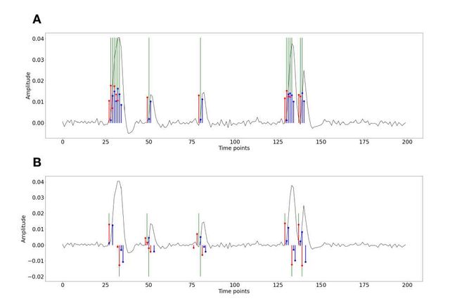
Figure S1: Activity-inducing (A) and innovation (B) signals estimated with PFM (red) and TA (blue) using their built-in HRF as opposed to using the same. The black line depicts the simulated signal, while the green lines indicate the onsets of the simulated neuronal events. X axis shows time in TRs.
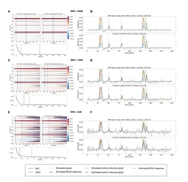
Figure S2: Spike model simulations. (Left) Heatmap of the regularization paths of the activity-inducing signal estimated with PFM and TA as a function of λ (increasing number of iterations in x-axis), whereas each row in the y-axis shows one time-point. Vertical lines denote iterations corresponding to the Akaike and Bayesian Information Criteria (AIC and BIC) optima. (Right) Estimated activity-inducing (blue) and activity-related (green) signals when set based on BIC. All estimates are identical, regardless of SNR.
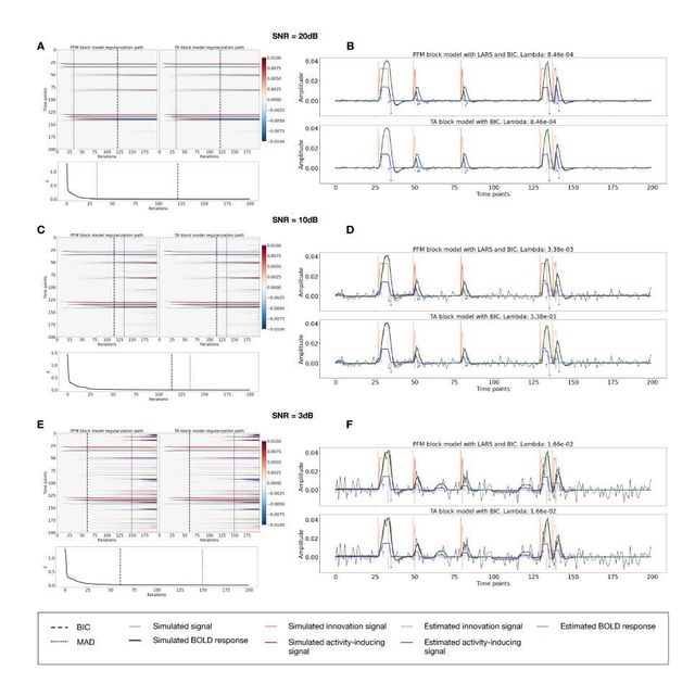
Figure S3: Block model simulations. (Left) Heatmap of the regularization paths of the innovation signal estimated with PFM and TA as a function of λ (increasing number of iterations in x-axis), whereas each row in the y-axis illustrates one time-point. Vertical lines denote iterations corresponding to the Akaike and Bayesian Information Criteria (AIC and BIC) optima. (Right) Estimated innovation (blue) and activity-related (green) signals when is set based on BIC. All the estimates are identical when compared between the PFM and TA cases, regardless of SNR.
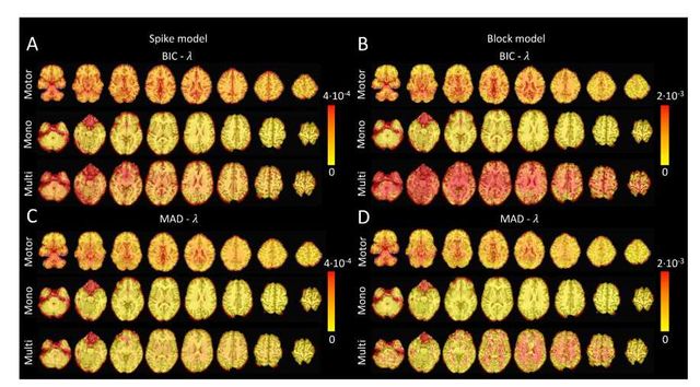
Figure S4: Values of λ across the different voxels in the brain used to estimate (A) the activity-inducing signal (spike model) and (B) the innovation signal (block model) with the BIC selection, as well as (C) the activity-inducing signal (block model) and (D) the innovation signal (block model) with a MAD-based selection. The λ maps are shown for the three experimental fMRI datasets: the motor task (Motor), the monoband resting-state (Mono), and the multiband resting-state (Multi) datasets.
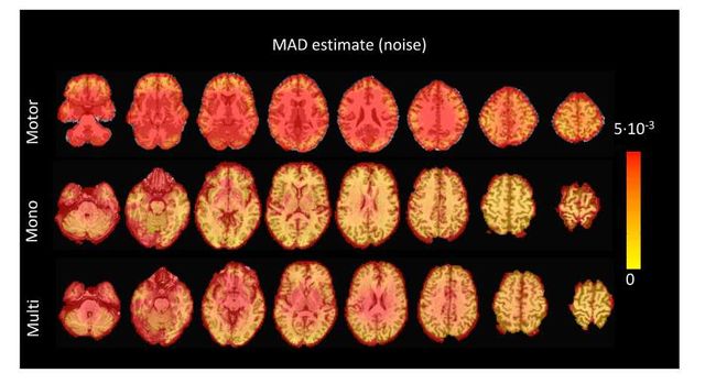
Figure S5: Values of the MAD estimate of standard deviation of the noise across the different voxels in the brain for the three experimental fMRI datasets: the motor task (Motor), the monoband resting-state (Mono), and the multiband resting-state (Multi) datasets.
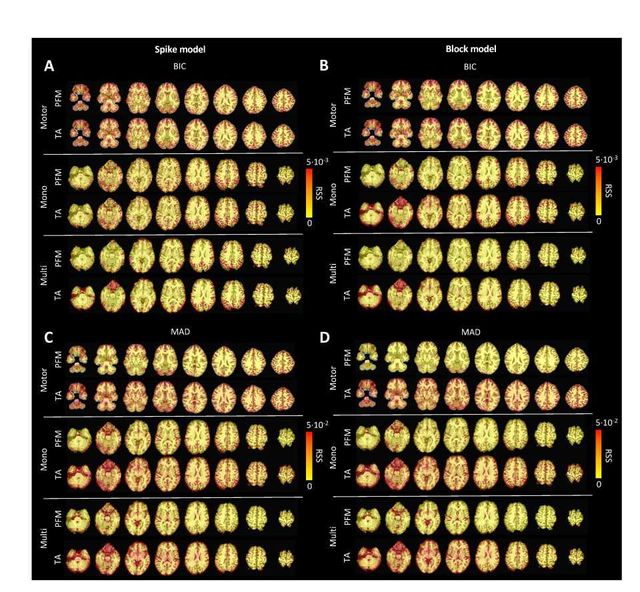
Figure S6: Root sum of squares (RSS) comparison between Paradigm Free Mapping and Total Activation for the three experimental fMRI datasets: the motor task (Motor), the monoband resting-state (Mono), and the multiband resting-state (Multi) datasets. RSS maps are shown for the spike (left) and block (right) models solved with a selection of λ based on the BIC (top) and MAD (bottom) criteria.
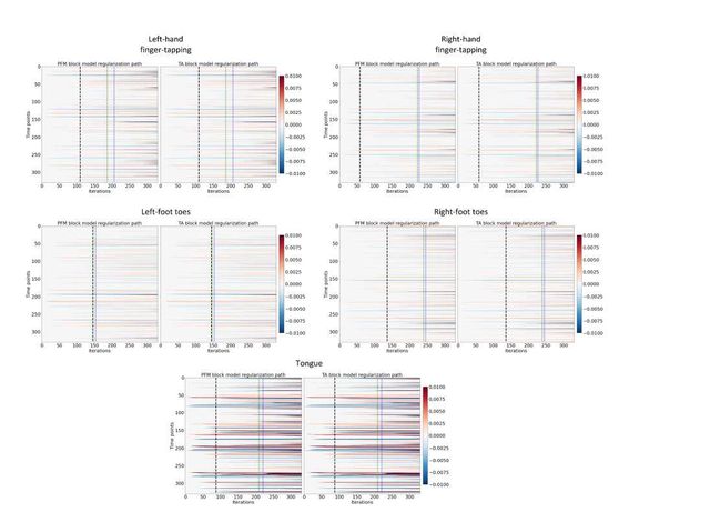
Figure S7: Regularization paths of the innovation signal estimated with PFM and TA as a function of λ (increasing number of iterations in x-axis, whereas each row in the y-axis shows one time-point) for the representative voxels of the motor task shown in Figure 5. Vertical lines denote selections of λ corresponding to the BIC (black), MAD based on LARS residuals (blue) and MAD based on FISTA residuals (green) optima.
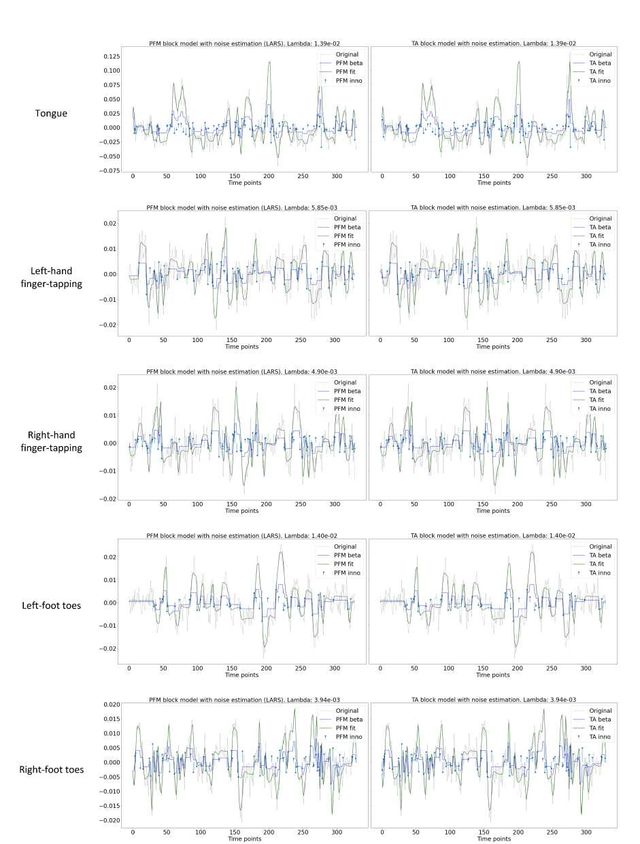
Figure S8: Estimated innovation signal (blue) and activity-related signal (green) for the representative voxels of the motor task shown in Figure 5 with the MAD selection of λ made by TA, i.e., employing the same λ with both PFM and TA.
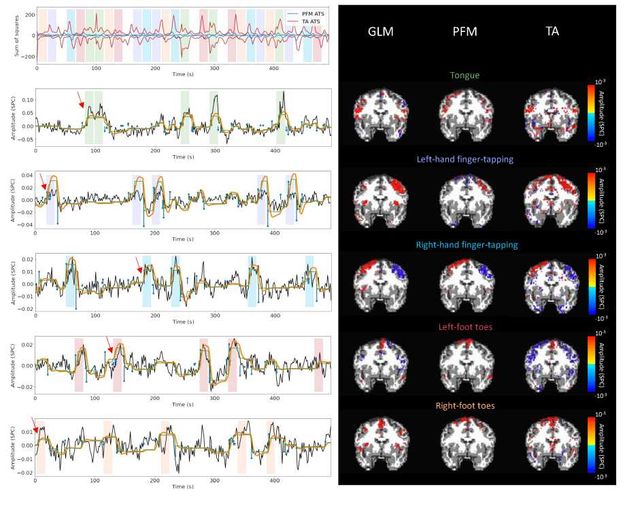
Figure S9: Activity maps of the motor task using a seletion of λ based on the MAD estimate. Row 1: Activation time-series of the innovation signals estimated by PFM (in blue) or TA (in red) calculated as the sum of squares of all voxels at every timepoint. Positive-valued and negative-valued contributions were separated into two distinct time-courses. Color-bands indicate the onset and duration of each condition in the task (green: tongue, purple: left-hand finger-tapping, blue: right-hand finger-tapping, red: left-foot toes, orange: right-foot toes). Rows 2–6: time-series of a representative voxel for each task with the PFM-estimated innovation (blue), PFM-estimated activity-inducing (green), and activity-related (i.e., fitted, orange) signals, with their corresponding GLM, PFM, and TA maps on the right. The maps shown on the right are sampled at the time-point labeled with the red arrows and display the innovation signals at that moment across the whole brain.
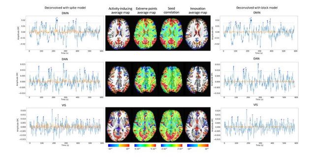
Figure S10: Activity-inducing CAPs (left) and innovation CAPs (right) obtained with the PFM-estimated activity-inducing and innovation signals respectively, using a MAD-based selection of λ. Time-points selected with a 95th percentile threshold are shown over the average time-series (blue) in the seed region (white-cross) and the deconvolved signal (orange). CAPs and seed correlation maps are illustrated in the center.
Summary
Ryan Dix
Metadata
Type of Research Object: